---
title: "Week 5 Practice Problems: Solutions"
author:
name: Alex Kaizer
roles: "Instructor"
affiliation: University of Colorado-Anschutz Medical Campus
toc: true
toc_float: true
toc-location: left
format:
html:
code-fold: show
code-overflow: wrap
code-tools: true
---
```{r, echo=F, message=F, warning=F}
library(kableExtra)
library(dplyr)
```
This page includes the solutions to the optional practice problems for the given week. If you want to see a version [without solutions please click here](/labs/prac5/index.qmd). Data sets, if needed, are provided on the BIOS 6618 Canvas page for students registered for the course.
This week's extra practice exercises are focusing on implementing bootstrap resampling and permutation testing to evaluate the odds ratio of an estimate.
# Data Background
Complete the following exercises to conduct a bootstrap and a permutation test for a data set we first used in last week's lab.
The following code can load the `Surgery_Timing.csv` file into R directly from our Canvas course. The surgery time data is based on a retrospective observational study of 32,001 elective general surgical patients, but we will subset to arthroplasty knee procedures. We will create a new variable to specify morning vs. afternoon surgery time as our "exposure" and will examine in-hospital complication rate as our "outcome" of interest.
```{r, cache=T, class.source = 'fold-show'}
dat1 <- read.csv('../../.data/Surgery_Timing.csv')
dat1s <- dat1[which(dat1$ahrq_ccs=='Arthroplasty knee'),]
dat1s$AK_morning <- dat1s$hour < 12 # create new variable for morning observation, I use the "AK_" prefix to indicate variables I created
```
With this information we can calculate the odds ratio in a few ways (manually, with a function, etc.):
```{r, message=FALSE, class.source = 'fold-show', warning=F}
# calculate the OR from epi.2by2
library(epiR)
tab1 <- table(morning = factor(dat1s$AK_morning, levels=c(TRUE,FALSE)), complication = factor(dat1s$complication, levels=c(1,0)) )
epi.2by2(tab1)
# calculate the OR by hand where OR = ad/bc
a <- sum( dat1s$AK_morning==T & dat1s$complication==1 )
b <- sum( dat1s$AK_morning==T & dat1s$complication==0 )
c <- sum( dat1s$AK_morning==F & dat1s$complication==1 )
d <- sum( dat1s$AK_morning==F & dat1s$complication==0 )
obs_or <- (a*d)/(b*c)
obs_or
```
We see that in both approaches we arrive at an estimated odds ratio of 0.844, with a 95% CI from `epi.2by2` of (0.63, 1.13).
## Exercise 1: Bootstrap Confidence Intervals
Estimate the 95% normal percentile and bootstrap percentile confidence intervals with 10,000 bootstrap samples to describe the variability of our estimate and:
**a.** compare the resulting CIs to the estimate from `epi.2by2`
**b.** evaluate if the normal percentile CI has acceptable coverage
**c.** evaluate if the bootstrap percentile CI has acceptable accuracy
**Solution:**
Let's start by implementing our bootstrap:
```{r}
B <- 10^4 #set number of bootstraps
or_boot <- numeric(B) #initialize vector to store results in

nM <- sum(dat1s$AK_morning==T) #sample size of morning knee procedures
nA <- sum(dat1s$AK_morning==F) #sample size of afternoon knee procedures

set.seed(1013) #set seed for reproducibility

for (i in 1:B){
    morning.boot <- sample(dat1s[which(dat1s$AK_morning==T),'complication'], nM, replace=T)
    afternoon.boot <- sample(dat1s[which(dat1s$AK_morning==F),'complication'], nM, replace=T)
    a <- sum( morning.boot==1 )
    b <- sum( morning.boot==0 )
    c <- sum( afternoon.boot==1 )
    d <- sum( afternoon.boot==0 )
    or_boot[i] <- (a*d)/(b*c)
}
```
Let's now visualize the shape of our bootstrap distribution:
```{r}
par(mfrow=c(1,2)) #create plotting area for 2 figures in one row
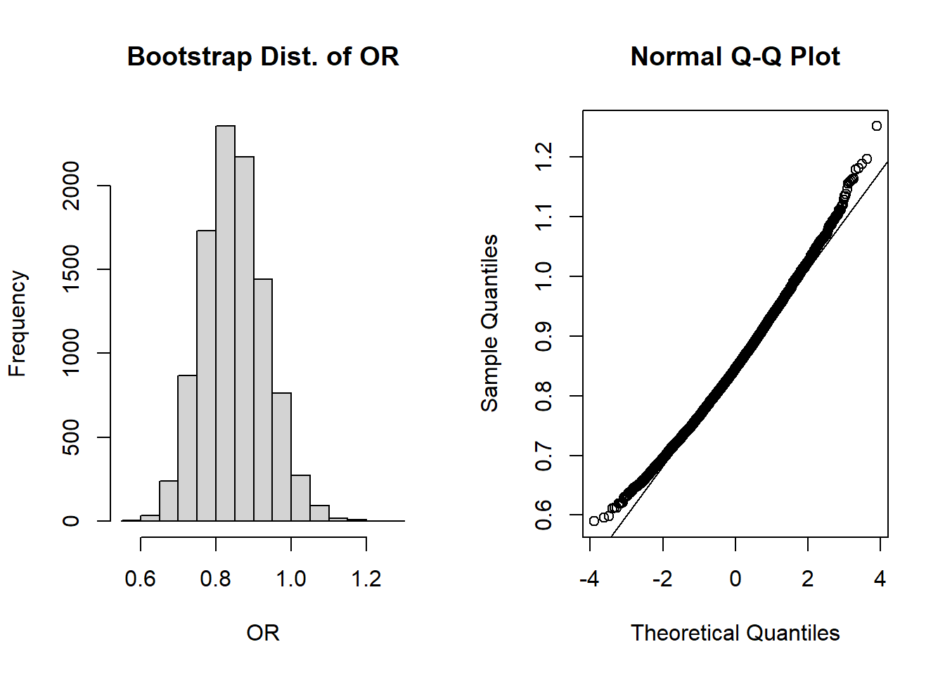
hist(or_boot, main='Bootstrap Dist. of OR', xlab='OR')
qqnorm(or_boot); qqline(or_boot)
```
The shapes of these plots suggest the odds ratios are NOT normally distributed, but are right skewed. However, recall that in our "by hand" confidence interval calculation we use $log(OR)$, so perhaps we can take a quick detour to see the plots on the log-scale:
```{r}
par(mfrow=c(1,2)) #create plotting area for 2 figures in one row
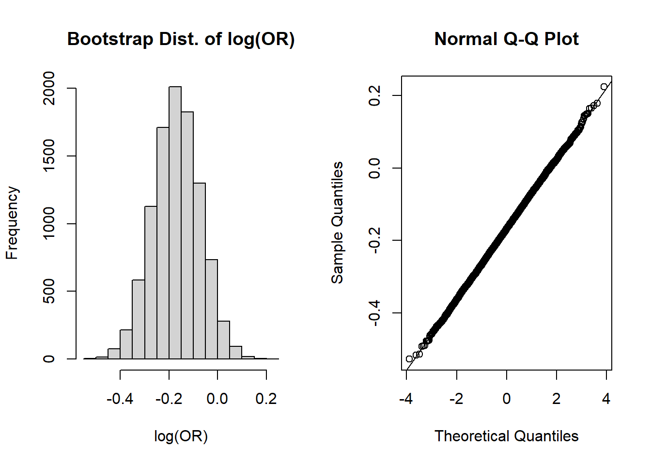
hist(log(or_boot), main='Bootstrap Dist. of log(OR)', xlab='log(OR)')
qqnorm(log(or_boot)); qqline(log(or_boot))
```
These look more normally distributed on the log scale (hence our use of the transformation).
*Now back from our detour to the plots of log(OR)!* Let's first calculate the 95% normal percentile CI and its coverage:
```{r}
# Lower limit and coverage
LL <- mean(or_boot) - 1.96*sd(or_boot)
LL
sum(or_boot < LL)/B # Coverage of CI at lower end
# Upper limit and coverage
UL <- mean(or_boot) + 1.96*sd(or_boot)
UL
sum(or_boot > UL)/B # Coverage of CI at upper end
```
Then let's calculate the 95% bootstrap percentile CI and its accuracy:
```{r, class.source = 'fold-show'}
mean(or_boot) # bootstrap mean OR
mean(or_boot)-obs_or # bias for OR
sd(or_boot) # bootstrap SE
(mean(or_boot)-obs_or) / sd(or_boot) # estimate of accuracy
quantile(or_boot, c(0.025,0.975)) # 95% bootstrap percentile CI
```
**Solution Part a:**
The 95% normal percentile CI is (0.686, 1.012), the 95% bootstrap percentile CI is (0.697, 1.020), and our 95% CI from `epi.2by2` was (0.63, 1.13). Both of these seem to suggest that our bootstrap estimates of the CIs on the OR-scale are biased towards the null compared the 95% confidence interval from `epi.2by2` (i.e., 0.686 and 0.697 are closer to 1 than the `epi.2by2` estimate of 0.63; 1.012 and 1.020 are closer to 1 than the `epi.2by2` estimate of 1.13).
*As yet another detour,* what if we calculated the 95% intervals on the log-scale and then exponentiated back to the OR scale (like we do when we calculate our 95% CI by hand):
```{r, collapse=T}
### 95% normal percentile CI on the log(OR) scale then exponentiated
# Lower limit and coverage
logLL <- mean(log(or_boot)) - 1.96*sd(log(or_boot))
expLL <- exp(logLL)
expLL
sum(or_boot < expLL)/B # Coverage of CI at lower end
# Upper limit and coverage
logUL <- mean(log(or_boot)) + 1.96*sd(log(or_boot))
expUL <- exp(logUL)
expUL
sum(or_boot > expUL)/B # Coverage of CI at upper end
### 95% bootstrap percentile CI on the log(OR) scale then exponentiated
exp( quantile(log(or_boot), c(0.025,0.975)) ) # 95% bootstrap percentile CI
```
There are few interesting points we can draw from this result:
* The normal percentile interval estimated in this way has better coverage (2.52% on the lower tail, 2.34% on the upper tail), and its 95% interval is (0.698, 1.023). So while the interval here and from `epi.2by2` still don't match very well, the coverage is improved when using the $log(OR)$ to estimate the interval. This "disconnect" between calculating the odds ratio at each iteration versus the log odds ratio is a direct application of [Jensen's inequality](https://en.wikipedia.org/wiki/Jensen%27s_inequality), where here we see that the exponentiated mean of log(OR) is not equivalent to the mean of the exponentiated log(OR) [i.e., the mean of our OR's].
* The bootstrap percentile interval is *unchanged* from before. This is because when calculating the quantiles, taking the log doesn't change the ordering or affect our estimates of the mean or standard error like it does in the normal percentile interval. So the estimate for $log(OR)$ and $OR$ have the same ordering (from smallest to largest), and our nonparametric estimate is unaffected.
**NOTE: This does not mean that the CI from the `epi.2by2` function is "wrong" or that our bootstrap estimates are "wrong"! Just that different approaches (and assumptions behind the approaches) can result in different estimates.**
**Solution Part b:**
In our original estimate on the original scale, the coverage is too low on the lower end (`LL`) at 1.7% (versus the expected 2.5% if normality held) and too high on the upper end (`UL`) at 3.21% (vs. 2.5%).
**Solution Part c:**
The ratio of |bias/SE| is less than 0.10, so we expect the bootstrap percentile CI to have acceptable accuracy.
## Exercise 2: Permutation Test P-value
Implement a permutation test with 10,000 resamples to estimate a p-value for if our observed OR is significantly different from its null value for:
**a.** a two-sided p-value.
**b.** a one-sided p-value where we hypothesize that mornings have a lower odds of complications compared to the afternoon.
**Solution:**
We will start by implementing our permutation test:
```{r}
B <- 10^4 - 1 #set number of times to complete permutation sampling
result <- numeric(B)

nM <- sum(dat1s$AK_morning==T) #sample size of morning knee procedures

a <- sum( dat1s$AK_morning==T & dat1s$complication==1 )
b <- sum( dat1s$AK_morning==T & dat1s$complication==0 )
c <- sum( dat1s$AK_morning==F & dat1s$complication==1 )
d <- sum( dat1s$AK_morning==F & dat1s$complication==0 )
obs_or <- (a*d)/(b*c) # the observed OR calculated manually

set.seed(1013) #set seed for reproducibility
pool_dat <- dat1s$complication

for(j in 1:B){
    index <- sample(x=1:length(pool_dat), size=nM, replace=F)
    morning_permute <- pool_dat[index]
    afternoon_permute <- pool_dat[-index]
    a <- sum( morning_permute==1 ) # calculate each cell of our 2x2 table to calculate the OR
    b <- sum( morning_permute==0 )
    c <- sum( afternoon_permute==1 )
    d <- sum( afternoon_permute==0 )
    result[j] <- (a*d)/(b*c)
}
```
We finish by visualizing our results:
```{r}
# Histogram
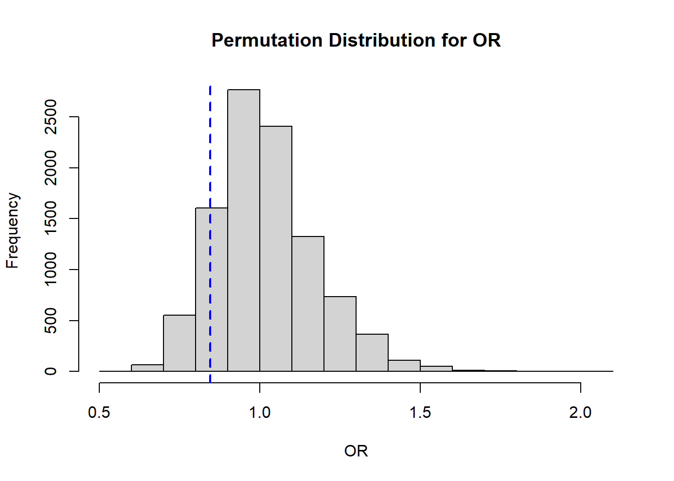
hist( result, xlab='OR',
main='Permutation Distribution for OR')
abline( v=obs_or, lty=2, col='blue', lwd=2)
```
**Solution Part a:**
Based on our permutation distribution, we will calculate the proportion that would fall into either tail, then multiply the larger value by 2 (to be more conservative):
```{r}
#note, we take the larger p-value and multiply by 2 (as compared to replacing <= with >)
((sum(result <= obs_or) + 1)/(B+1))
((sum(result >= (1/obs_or)) + 1)/(B+1))
```
Here we see that the larger value is 0.1644, so our estimated 2-sided p-value is `r 2*max(((sum(result >= (1/obs_or)) + 1)/(B+1)),((sum(result <= obs_or) + 1)/(B+1)))`. Therefore we would fail to reject the null hypothesis that the OR=1.
**Solution Part b:**
In this case, we have *a priori* specified a one-sided test, so we can evaluate the proportion of our permutation distribution that falls below our observed OR of 0.844 from **2a**. Here we see $p=0.1408$, so we still fail to reject $H_0$ that the odds of a complication are different between morning and afternoon in knee surgeries.