Week 9 Practice Problems: Solutions

Author

Affiliation

Alex Kaizer

University of Colorado-Anschutz Medical Campus

This page includes the solutions to the optional practice problems for the given week. If you want to see a version without solutions please click here. Data sets, if needed, are provided on the BIOS 6618 Canvas page for students registered for the course.

This week’s extra practice exercises are focusing on implementing and interpreting a multiple linear regression (MLR) model, both using existing functions and by coding our own matrices.

Dataset Background

The following code can load the Licorice_Gargle.csv file into R:

dat_all <- read.csv('../../.data/Licorice_Gargle.csv')

# remove records with missing data for the outcome or any predictors:
complete_case_vec <- complete.cases(dat_all[,c('pacu30min_throatPain','preOp_gender','preOp_age','treat')]) # creates a vector of TRUE or FALSE for each row if the cases are complete (i.e., no NA values)
dat <- dat_all[complete_case_vec,]

The dataset represents a randomized control trial of 236 adult patients undergoing elective thoracic surgery requiring a double-lumen endotracheal tube comparing if licorice vs. sugar-water gargle prevents postoperative sore throat. For our exercises below we will focus on the following variables:

• pacu30min_throatPain: sore throat pain score at rest 30 minutes after arriving in the post-anesthesia care unit (PACU) measured on an 11 point Likert scale (0=no pain to 10=worst pain)
• preOp_gender: an indicator variable for gender (0=Male, 1=Female)
• preOp_age: age (in years)
• treat: the randomized treatment in the trial where 0=sugar 5g and 1=licorice 0.5g

For our solutions, we will also use our ANOVA table creation function from lecture/recitation:

linreg_anova_func <- function(mod, ndigits=2, p_ndigits=3, format='kable'){
### Function to create an ANOVA table linear regression results from lm or glm
# mod: an object with the fitted model results
# ndigits: number of digits to round to for most values, default is 2
# p_digits: number of digits to round the p-value to, default is 3
# format: desired format output (default is kable):
## "kable" for kable table
## "df" for data frame as table

  # extract outcome from the object produced by the glm or lm function
  if( class(mod)[1] == 'glm' ){
    y <- mod$y
  }
  if( class(mod)[1] == 'lm' ){
    y <- mod$model[,1] # first column contains outcome data
  }  
  
  ybar <- mean(y)
  yhat <- predict(mod)
  p <- length(mod$coefficients)-1
  n <- length(y)

  ssm <- sum( (yhat-ybar)^2 )
  sse <- sum( (y-yhat)^2 )
  sst <- sum( (y-ybar)^2 )
  
  msm <- ssm/p
  mse <- sse/(n-p-1)
  
  f_val <- msm/mse
  p_val <- pf(f_val, df1=p, df2=n-p-1, lower.tail=FALSE)
  
  # Create an ANOVA table to summarize all our results:
  p_digits <- (10^(-p_ndigits))
  p_val_tab <- if(p_val<p_digits){paste0('<',p_digits)}else{round(p_val,p_ndigits)}
  
  anova_table <- data.frame( 'Source' = c('Model','Error','Total'),
                          'Sums of Squares' = c(round(ssm,ndigits), round(sse,ndigits), round(sst,ndigits)),
                          'Degrees of Freedom' = c(p, n-p-1, n-1),
                          'Mean Square' = c(round(msm,ndigits), round(mse,ndigits),''),
                          'F Value' = c(round(f_val,ndigits),'',''),
                          'p-value' = c(p_val_tab,'',''))

  if( format == 'kable' ){  
    library(kableExtra)
    kbl(anova_table, col.names=c('Source','Sums of Squares','Degrees of Freedom','Mean Square','F-value','p-value'), align='lccccc', escape=F) %>%
      kable_styling(bootstrap_options = "striped", full_width = F, position = "left")
  }else{
    anova_table
  }
}

Exercise 1: Multiple Linear Regression Example

1a: The True Regression Equation

Write the the multiple linear regression model for the outcome of throat pain (i.e., dependent variable) and independent variables for ASA score, gender, age, and treatment status. Be sure to define all terms.

Solution:

The true regression model is

\[ Y_i = \beta_0 + \beta_1 X_{\text{Licorice},i} + \beta_2 X_{\text{Female},i} + \beta_3 X_{\text{Age},i} + \epsilon_i \]

where \(\epsilon_i \sim N(0,\sigma^{2}_{Y|X})\) and the subscript for each variable corresponds to the designated variable (e.g., the group if categorical, or the value if continuous).

1b: Fitting the Model

Fit the multiple linear regression model for the outcome of throat pain (i.e., dependent variable) and independent variables for ASA score, gender, age, and treatment status. Print the summary table output for reference in the following questions.

Solution:

We could fit this model with either lm or glm:

# Fit with lm function
lm_full <- lm(pacu30min_throatPain ~ treat + preOp_gender + preOp_age, data=dat)
summary(lm_full)

Call:
lm(formula = pacu30min_throatPain ~ treat + preOp_gender + preOp_age, 
    data = dat)

Residuals:
    Min      1Q  Median      3Q     Max 
-1.1968 -0.8539 -0.3559  0.5968  5.1079 

Coefficients:
              Estimate Std. Error t value Pr(>|t|)    
(Intercept)   1.229559   0.317234   3.876 0.000139 ***
treat        -0.744559   0.156179  -4.767 3.32e-06 ***
preOp_gender -0.259238   0.159345  -1.627 0.105134    
preOp_age    -0.001819   0.005051  -0.360 0.719128    
---
Signif. codes:  0 '***' 0.001 '**' 0.01 '*' 0.05 '.' 0.1 ' ' 1

Residual standard error: 1.19 on 229 degrees of freedom
Multiple R-squared:  0.1023,    Adjusted R-squared:  0.09054 
F-statistic: 8.699 on 3 and 229 DF,  p-value: 1.728e-05

# Fit with glm function
glm_full <- glm(pacu30min_throatPain ~ treat + preOp_gender + preOp_age, data=dat)
summary(glm_full)

Call:
glm(formula = pacu30min_throatPain ~ treat + preOp_gender + preOp_age, 
    data = dat)

Coefficients:
              Estimate Std. Error t value Pr(>|t|)    
(Intercept)   1.229559   0.317234   3.876 0.000139 ***
treat        -0.744559   0.156179  -4.767 3.32e-06 ***
preOp_gender -0.259238   0.159345  -1.627 0.105134    
preOp_age    -0.001819   0.005051  -0.360 0.719128    
---
Signif. codes:  0 '***' 0.001 '**' 0.01 '*' 0.05 '.' 0.1 ' ' 1

(Dispersion parameter for gaussian family taken to be 1.415709)

    Null deviance: 361.14  on 232  degrees of freedom
Residual deviance: 324.20  on 229  degrees of freedom
AIC: 748.19

Number of Fisher Scoring iterations: 2

Notice, since we haven’t changed any of the variable types, it is treating treat and preOp_gender as numeric (i.e., it doesn’t specify the group in the variable name) since the values are 0/1. Since they are binary, we can see we arrive at identical results if we coerce the variables to categorical with as.factor():

# Fit with lm function but with treat and preOp_gender as factors
lm_full_factor <- lm(pacu30min_throatPain ~ as.factor(treat) + as.factor(preOp_gender) + preOp_age, data=dat)
summary(lm_full_factor)

Call:
lm(formula = pacu30min_throatPain ~ as.factor(treat) + as.factor(preOp_gender) + 
    preOp_age, data = dat)

Residuals:
    Min      1Q  Median      3Q     Max 
-1.1968 -0.8539 -0.3559  0.5968  5.1079 

Coefficients:
                          Estimate Std. Error t value Pr(>|t|)    
(Intercept)               1.229559   0.317234   3.876 0.000139 ***
as.factor(treat)1        -0.744559   0.156179  -4.767 3.32e-06 ***
as.factor(preOp_gender)1 -0.259238   0.159345  -1.627 0.105134    
preOp_age                -0.001819   0.005051  -0.360 0.719128    
---
Signif. codes:  0 '***' 0.001 '**' 0.01 '*' 0.05 '.' 0.1 ' ' 1

Residual standard error: 1.19 on 229 degrees of freedom
Multiple R-squared:  0.1023,    Adjusted R-squared:  0.09054 
F-statistic: 8.699 on 3 and 229 DF,  p-value: 1.728e-05

Since our later questions ask for a “brief, but complete” interpretation, we can also output the confidence intervals:

# Print confidence intervals to use for later responses
confint(lm_full)

                   2.5 %       97.5 %
(Intercept)   0.60448955  1.854629278
treat        -1.05229143 -0.436826568
preOp_gender -0.57320823  0.054731424
preOp_age    -0.01177002  0.008132942

1c: Predicted Regression Equation

Write down the predicted regression equation that describes the relationship between throat pain and your predictors based on the output.

Solution:

Our predicted regression equation is

\[ \hat{Y}_i = 1.230 + -0.745 X_{\text{Licorice},i} + -0.259 X_{\text{Female},i} + -0.002 X_{\text{Age},i} \]

1d: Intercept Interpretation and Hypothesis Test

Write the hypothesis being tested in the regression output for this coefficient. What is the estimated intercept and how would you interpret it (provide a brief, but complete, interpretation)?

Solution:

Our hypotheses are \(H_0\colon \beta_0 = 0\) versus \(H_1\colon \beta_0 \neq 0\).

The average throat pain after 30 minutes in the PACU is 1.230 (95% CI: 0.604, 1.855) when all other predictors are 0. Since p<0.001, we reject the null hypothesis and conclude it is significantly different from 0.

This interpretation, however, is nonsensical since it both extrapolates to ages we do not have (i.e., 0) and a newborn would not be able to report their pain at 30 minutes in the PACU.

Recall, our brief, but complete, interpretation involves (1) the point estimate, (2) an interval estimate, (3) a decision, and (4) a measure of uncertainty.

1e: Coefficient Interpretation and Hypothesis Test for Binary Predictor

Write the hypothesis being tested in the regression output for this coefficient. What is the estimated effect of treatment and how would you interpret it (provide a brief, but complete, interpretation)?

Solution:

Our hypotheses are \(H_0\colon \beta_1 = 0\) versus \(H_1\colon \beta_1 \neq 0\).

Those treated with licorice have a significantly lower throat pain score after 30 minutes in the PACU that is, on average, 0.745 lower (95% CI: 0.437 to 1.052 lower) than those treated with sugar water after adjusting for gender and age (p<0.001).

1f: Coefficient Interpretation and Hypothesis Test for Continuous Predictor

Write the hypothesis being tested in the regression output for this coefficient. What is the estimated effect of age and how would you interpret it (provide a brief, but complete, interpretation)?

Solution:

Our hypotheses are \(H_0\colon \beta_3 = 0\) versus \(H_1\colon \beta_3 \neq 0\).

For a one year increase in age, throat pain score after 30 minutes in the PACU is 0.002 higher (95% CI: -0.012 lower to 0.008 higher) after adjusting for treatment group and gender. Since p=0.719, we fail to reject the null hypothesis that the slope is different from 0.

1g: The Partial F-test

Evaluate if the addition of age and gender contribute significantly to the prediction of throat pain over and above that achieved by treatment group alone. Write out the null and alternative hypotheses being tested and your conclusion.

Solution:

We can do this “by hand” or using R (or SAS) to do the calculations for us. We will start with our hand calculation and compare to R’s result.

The null hypothesis we are evaluating is \(H_0\colon \beta_2 = \beta_3 = 0\) versus the alternative hypothesis (\(H_1\)) that at least one coefficient of \(\beta_2\) and \(\beta_3\) is not equal to 0.

First, we must fit the reduced model and create the ANOVA tables for both the full and reduced models:

# Create ANOVA table for full model
linreg_anova_func(lm_full)

Source	Sums of Squares	Degrees of Freedom	Mean Square	F-value	p-value
Model	36.94	3	12.31	8.7	<0.001
Error	324.20	229	1.42
Total	361.14	232

# Fit reduced model with age and gender removed
lm_red <- lm(pacu30min_throatPain ~ treat, data=dat)

# Create ANOVA table for reduced model
linreg_anova_func(lm_red)

Source	Sums of Squares	Degrees of Freedom	Mean Square	F-value	p-value
Model	32.97	1	32.97	23.21	<0.001
Error	328.17	231	1.42
Total	361.14	232

Taking the relevant quantities from our ANOVA tables, we can calculate our partial \(F\) statistic:

\[ F = \frac{SS_{model}(full) - SS_{model}(reduced)]/k}{MS_{error}(full)} = \frac{(36.94 - 32.97) / 2}{1.42} = 1.40 \sim F_{2,233-1-2-1} = F_{2,229} \]

Since we are using software, we can calculate the p-value directly that \(P(F \geq F_{2,229})\) using pf(1.40,2,229,lower.tail=F): 0.249. Since we see that p>0.05, we fail to reject the null hypothesis that the addition of age and gender contribute significantly to the prediction of throat pain over and above that achieved by treatment group alone.

Another approach we could use is to calculate the critical value represented by \(F_{2,229}\) for an \(\alpha=0.05\) to compare our test statistic to using qf(0.95,2,229): 3.035. Since \(F=1.40 < 3.035 = F_{0.95,2,229}\), we would still fail to reject our null hypothesis.

A third approach would be to use the anova function in R to solve this without doing any calculations by hand:

anova(lm_full, lm_red, test='F')

Analysis of Variance Table

Model 1: pacu30min_throatPain ~ treat + preOp_gender + preOp_age
Model 2: pacu30min_throatPain ~ treat
  Res.Df    RSS Df Sum of Sq      F Pr(>F)
1    229 324.20                           
2    231 328.17 -2   -3.9728 1.4031 0.2479

We see our results closely match our by hand work above (with some slight differences due to rounding), where we still have \(p>0.05\) and fail to reject the null hypothesis.

1h: The Overall F-test

Evaluate if the the entire set of independent variables (i.e., predictors) contribute significantly to the prediction of throat pain. Write out the null and alternative hypotheses being tested and your conclusion.

Solution:

The null hypothesis is that \(H_0\colon \beta_1 = \beta_2 = \beta_3 = 0\) versus the alternative hypothesis (\(H_1\)) that at least one of these \(\beta_k; k=1,2,3\) is not equal to 0.

For this problem, we can see that in our lm_full summary that \(F=8.699\) and its corresponding \(p<0.001\). Since \(p<0.05\), we reject the null hypothesis and conclude that at least one \(\beta_k\) is significantly different from 0.

Further, we could combine our findings from the previous problem to note that adding age and gender were not significant, so it seems that a model with just treatment would be better and more parsimonious, even if the overall \(F\)-test for all three predictors is significant.

1i: Multicollinearity

Calculate the variance inflation factors (VIFs) for the independent variables in the model. Does it appear that multicollinearity may be a concern?

Solution:

car::vif(lm_full)

       treat preOp_gender    preOp_age 
    1.003602     1.002208     1.002467 

Since all VIFs are less than 10, it appears multicollinearity is not a concern in our full model.

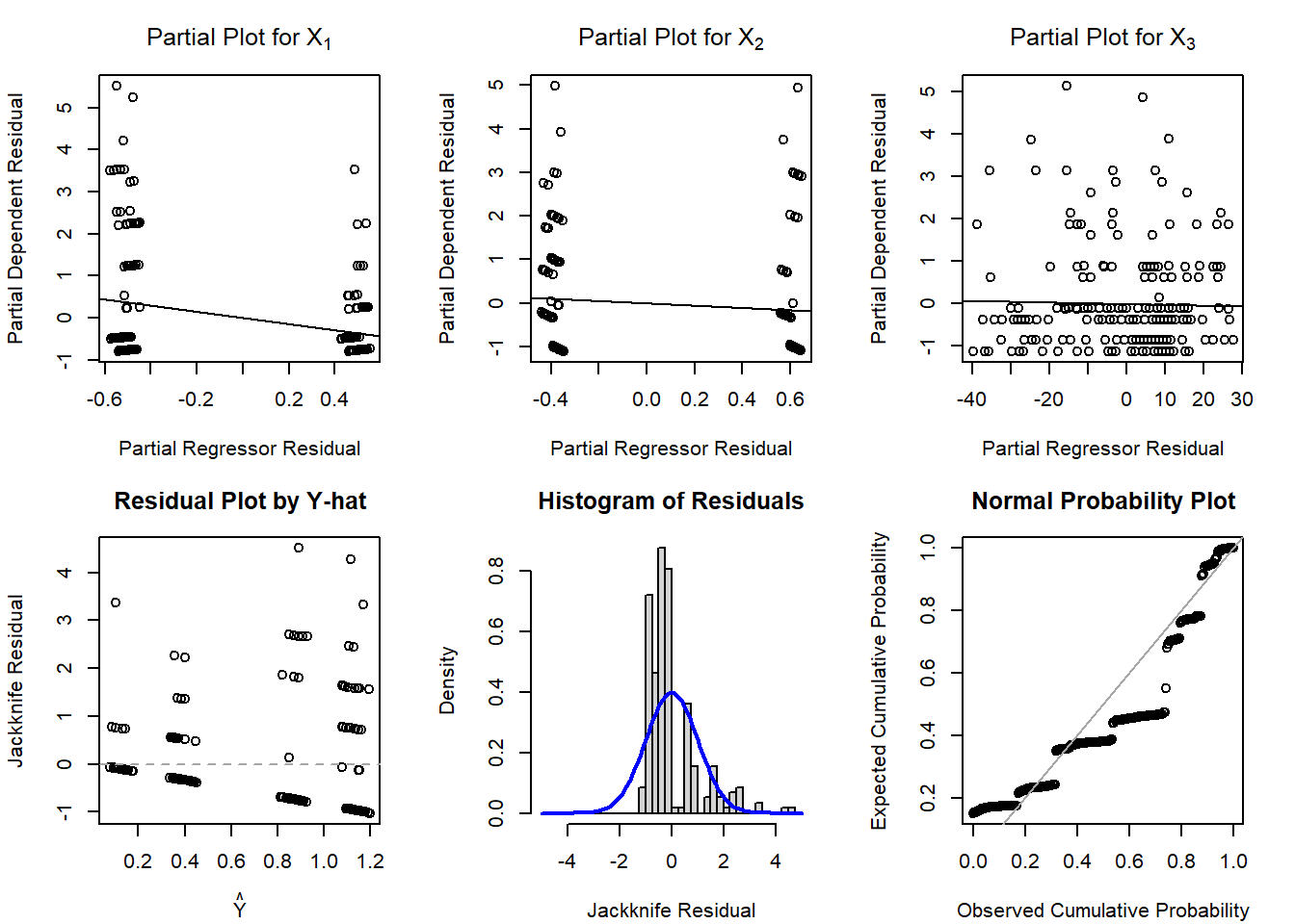
1j: Diagnostic Plots

Evaluate the assumptions of our multiple linear regression model by creating diagnostic plots.

Solution:

par(mfrow=c(2,3), mar=c(4.1,4.1,3.1,2.1))

## X1 Partial Plot MLR
x1_mlr_step1 <- lm(pacu30min_throatPain ~ preOp_gender + preOp_age, data=dat)
x1_mlr_step2 <- lm(treat ~ preOp_gender + preOp_age, data=dat)
plot(x=residuals(x1_mlr_step2), y=residuals(x1_mlr_step1),
     main=expression('Partial Plot for X'[1]), ylab='Partial Dependent Residual', 
     xlab='Partial Regressor Residual')
abline(lm(residuals(x1_mlr_step1) ~ residuals(x1_mlr_step2)))


## X2 Partial Plot MLR
x2_mlr_step1 <- lm(pacu30min_throatPain ~ treat + preOp_age, data=dat)
x2_mlr_step2 <- lm(preOp_gender ~ treat + preOp_age, data=dat)
plot(x=residuals(x2_mlr_step2), y=residuals(x2_mlr_step1),
     main=expression('Partial Plot for X'[2]), ylab='Partial Dependent Residual', 
     xlab='Partial Regressor Residual')
abline(lm(residuals(x2_mlr_step1) ~ residuals(x2_mlr_step2)))


## X3 Partial Plot MLR
x3_mlr_step1 <- lm(pacu30min_throatPain ~ treat + preOp_gender, data=dat)
x3_mlr_step2 <- lm(preOp_age ~ treat + preOp_gender, data=dat)
plot(x=residuals(x3_mlr_step2), y=residuals(x3_mlr_step1),
     main=expression('Partial Plot for X'[3]), ylab='Partial Dependent Residual', 
     xlab='Partial Regressor Residual')
abline(lm(residuals(x3_mlr_step1) ~ residuals(x3_mlr_step2)))


## Scatterplot of residuals by predicted values
plot(x=predict(lm_full), y=rstudent(lm_full), xlab=expression(hat(Y)), ylab='Jackknife Residual', 
     main='Residual Plot by Y-hat', cex=1); abline(h=0, lty=2, col='gray65')

## Histogram of jackknife residuals with normal curve
hist(rstudent(lm_full), xlab='Jackknife Residual', 
     main='Histogram of Residuals', freq=F, breaks=seq(-5,5,0.25)); 
  curve( dnorm(x,mean=0,sd=1), lwd=2, col='blue', add=T)

## PP-plot
plot( ppoints(length(rstudent(lm_full))), sort(pnorm(rstudent(lm_full))), 
      xlab='Observed Cumulative Probability', 
      ylab='Expected Cumulative Probability', 
      main='Normal Probability Plot', cex=1); 
  abline(a=0,b=1, col='gray65', lwd=1)

These plots are somewhat challenging to decipher since we have two categorical predictors and only one continuous predictor. However, the lower figures all suggest that normality may be violated and that this model, as it currently is, may not be the most appropriate. It is possible that a data transformation may result in a model more appropriate for linear regression. Adding other variables (that may or may not be measured), may also improve the model fit. It is also entirely possible that our outcome of a 0-10 Likert pain scale is not normal and an entirely different approach to modeling may be needed (e.g., zero-inflated Poisson regression).

Exercise 2: But Now With Matrices!

Using your results in Exercise 1 to check your answers, complete the following parts using matrices you code yourself.

2a: The Design Matrix

Create the design matrix that we will use for our regression calculations.

Solution:

Our design matrix, \(\mathbf{X}\), includes a columns of 1’s for the intercept and then our three predictors:

X <- as.matrix( cbind(1, dat[,c('treat','preOp_gender','preOp_age')]) )

2b: Beta Coefficients

Calculate the estimated beta coefficients via matrix algebra.

Solution:

We need to first create a vector for our outcome of throat pain (Y). Then we will calculate \(\hat{\boldsymbol{\beta}} = (\mathbf{X}^\top\mathbf{X})^{-1}\mathbf{X}^\top\mathbf{Y}\):

Y <- dat$pacu30min_throatPain
beta_est <- solve(t(X) %*% X) %*% t(X) %*% Y
beta_est

                     [,1]
1             1.229559412
treat        -0.744558998
preOp_gender -0.259238404
preOp_age    -0.001818539

We see that our estimates match those from the lm function.

2c: Standard Error of Beta Coefficients

Calculate the standard error of the beta coefficients via matrix algebra.

Solution:

We will first calculate our MSE as \(\hat{\sigma}_{Y|X}^{2} = \frac{SSE}{n-p-1} = \frac{\mathbf{Y}^\top\mathbf{Y}-\hat{\boldsymbol{\beta}}^\top\mathbf{X}^\top\mathbf{Y}}{n-p-1}\):

mse <- (t(Y) %*% Y - t(beta_est) %*% t(X) %*% Y) / (nrow(dat) - ncol(X))
mse

         [,1]
[1,] 1.415709

Notice, that \(n-p-1\) can be pulled from our objects as \(n=\)nrow(dat) and \(p-1=\)ncol(X) (since our design matrix already includes the intercept).

The variance of our beta coefficients is therefore \(Var(\hat{\boldsymbol{\beta}}) = \hat{\sigma}_{Y|X}^{2} (\mathbf{X}^\top \mathbf{X})^{-1}\), which is our variance-covariance matrix:

beta_var <- as.numeric( mse ) * solve(t(X) %*% X)
beta_var

                        1         treat  preOp_gender     preOp_age
1             0.100637153 -1.384092e-02 -8.509392e-03 -1.470583e-03
treat        -0.013840916  2.439202e-02 -1.028729e-03  3.498007e-05
preOp_gender -0.008509392 -1.028729e-03  2.539084e-02 -1.935834e-05
preOp_age    -0.001470583  3.498007e-05 -1.935834e-05  2.550802e-05

We can compare this to the vcov output:

vcov(lm_full)

              (Intercept)         treat  preOp_gender     preOp_age
(Intercept)   0.100637153 -1.384092e-02 -8.509392e-03 -1.470583e-03
treat        -0.013840916  2.439202e-02 -1.028729e-03  3.498007e-05
preOp_gender -0.008509392 -1.028729e-03  2.539084e-02 -1.935834e-05
preOp_age    -0.001470583  3.498007e-05 -1.935834e-05  2.550802e-05

The standard error is then the square root of the variance terms along the diagonal:

beta_se <- sqrt(diag(beta_var))
beta_se

           1        treat preOp_gender    preOp_age 
 0.317233593  0.156179445  0.159345030  0.005050546 

This matches our lm output.

2d: Test Statistics and p-values

Calculate the \(t\)-statistic and associated p-value based on the previous estimates from 1b and 1c.

Solution:

We know that our \(t\)-statistic is the beta coefficient estimate divided by its standard error:

t_stat <- beta_est / beta_se
t_stat

                   [,1]
1             3.8758802
treat        -4.7673303
preOp_gender -1.6268998
preOp_age    -0.3600678

The p-value is then calculated for our two-sided test:

pval <- 2 * (1-pt( abs(t_stat), df = length(Y) - ncol(X)) ) # df = n-p-1
pval

                     [,1]
1            1.387762e-04
treat        3.319843e-06
preOp_gender 1.051336e-01
preOp_age    7.191283e-01

These results match the p-values in our regression output.

2e: Confidence and Prediction Interval

Calculate the 95% confidence and prediction interval for a male in the treatment group who is 50 years old. Compare this result to the calculation provided by R when using the predict function.

Solution:

We first need to define \(x_0\) for our given combination of covariates:

x0 <- c(1,1,0,50) # intercept, treatment, gender, age
pred_val <- t(x0) %*% beta_est # predicted throat pain score
pred_val

          [,1]
[1,] 0.3940735

We can then calculate our variances for a predicted mean and individual value. The variance for a fitted value (i.e., the expected mean \(\mu\) for a given value of \(X=x_0\)) is given by \[ Var(\mu_{Y|x_0}) = x_0^\top [Var(\hat{\boldsymbol{\beta}})] x_0 = \hat{\sigma}^{2}_{Y|X} x_{0}^\top (\mathbf{X}^\top \mathbf{X})^{-1} x_{0} \]

The variance of a future predicted value of \(Y\) for a given \(x_0\) for an individual is given by: \[ Var(\hat{Y} | x_0 ) = \hat{\sigma}^{2}_{Y|X} \left[ 1 + x_{0}^\top (\mathbf{X}^\top \mathbf{X})^{-1} x_{0}\right] \]

var_mean <- t(x0) %*% beta_var %*% x0
var_ind <- as.numeric( mse ) * (1 + t(x0) %*% solve(t(X) %*% X) %*% x0)

The 95% confidence and prediction intervals are:

## Note, we don't necessarily need to wrap pred_val and var_mean or var_ind in as.numeric(), but it avoids a warning about deprecated functions
# 95% CI
as.numeric(pred_val) + qnorm(c(0.025,0.975)) * sqrt(as.numeric(var_mean))

[1] 0.1343719 0.6537750

# 95% PI
as.numeric(pred_val) + qnorm(c(0.025,0.975)) * sqrt(as.numeric(var_ind))

[1] -1.952378  2.740525

We can compare this to the predict function:

predict(lm_full, newdata = data.frame(treat=1, preOp_gender=0, preOp_age=50), interval='confidence')

        fit       lwr       upr
1 0.3940735 0.1329921 0.6551548

predict(lm_full, newdata = data.frame(treat=1, preOp_gender=0, preOp_age=50), interval='predict')

        fit       lwr      upr
1 0.3940735 -1.964845 2.752992

We see that our matrix approach and the lm::predict function nearly match. The difference being due to using the standard normal (\(Z\)) distribution instead of the \(t\)-distribution in our “by hand” calculation. If we use the \(t_{229}\) distribution instead, we see they do exactly match:

## Note, we don't necessarily need to wrap pred_val and var_mean or var_ind in as.numeric(), but it avoids a warning about deprecated functions
# 95% CI
as.numeric(pred_val) + qt(c(0.025,0.975), df=229) * sqrt(as.numeric(var_mean))

[1] 0.1329921 0.6551548

# 95% PI
as.numeric(pred_val) + qt(c(0.025,0.975), df=229) * sqrt(as.numeric(var_ind))

[1] -1.964845  2.752992