---
title: "Permutation Test p-values"
author:
name: Alex Kaizer
roles: "Instructor"
affiliation: University of Colorado-Anschutz Medical Campus
toc: true
toc_float: true
toc-location: left
format:
html:
code-fold: show
code-overflow: wrap
code-tools: true
---
```{r, echo=F, message=F, warning=F}
library(kableExtra)
library(dplyr)
```
This page is part of the University of Colorado-Anschutz Medical Campus' [BIOS 6618 Recitation](/recitation/index.qmd) collection. To view other questions, you can view the [BIOS 6618 Recitation](/recitation/index.qmd) collection page or use the search bar to look for keywords.
# Permutation Test p-values
Let's revisit the example from lab on Tuesday with a comparison of a vaccine for Celiac disease to more explicitly walk through how we calculate the p-values and what happens if something goes wrong. We assumed under the null scenario that the placebo group's tissue transglutaminase IgA antibody (tTG-IgA) distribution was $Y_P \sim \text{Gamma}(\text{shape}=10,\text{scale}=3)$ and that the treatment group's tTG-IgA was $Y_T \sim \text{Gamma}(\text{shape}=10,\text{scale}=\sqrt{18})$.
```{r, class.source = 'fold-show'}
set.seed(612)
placebo <- rgamma(n=50, shape=10, scale=3)
vaccine <- rgamma(n=50, shape=5, scale=sqrt(18))

var(placebo) # calculate the sample variances
var(vaccine) # calculate the sample variances
obs_ratio <- var(placebo)/var(vaccine) # calculate the ratio of the variances
obs_ratio
B <- 10^4 - 1 #set number of times to complete permutation sampling
result <- numeric(B)
nP <- length(placebo)
obs_ratio <- var(placebo)/var(vaccine) # calculate the ratio of the variances
set.seed(612) #set seed for reproducibility
pool_dat <- c(placebo, vaccine)
for(j in 1:B){
index <- sample(x=1:length(pool_dat), size=nP, replace=F)
placebo_permute <- pool_dat[index]
vaccine_permute <- pool_dat[-index]
result[j] <- var(placebo_permute) / var(vaccine_permute)
}
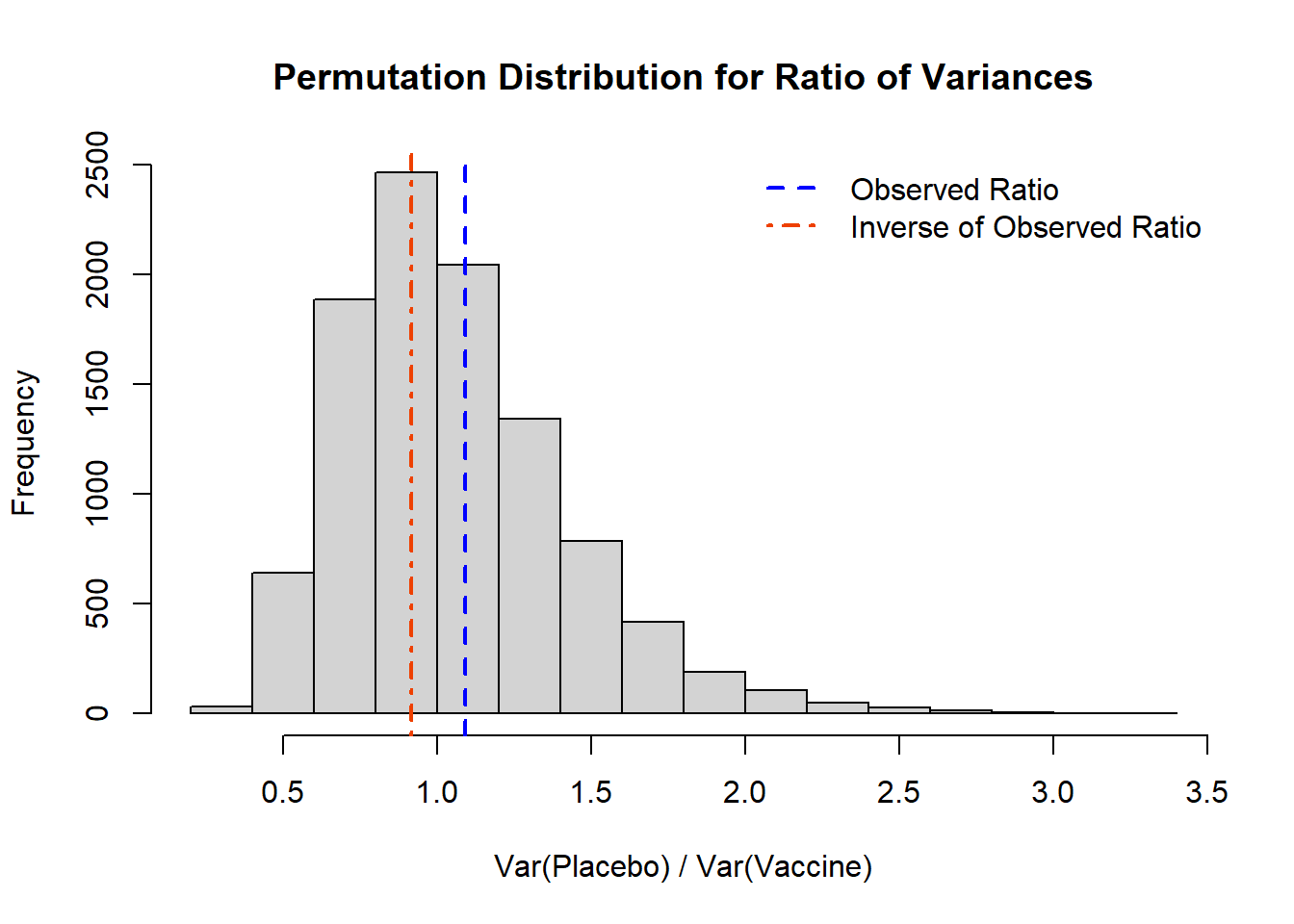
# Histogram
hist( result, xlab='Var(Placebo) / Var(Vaccine)',
main='Permutation Distribution for Ratio of Variances')
abline( v=obs_ratio, lty=2, col='blue', lwd=2)
abline( v=1/obs_ratio, lty=4, col='orangered2', lwd=2)
legend('topright', lty=c(2,4), lwd=c(2,2), col=c('blue','orangered2'), legend=c('Observed Ratio','Inverse of Observed Ratio'), bty='n')
```
We see in the histogram above that we have both the observed ratio (`obs_ratio`) and the inverse of our observed ratio (`1/obs_ratio`) indicated by the vertical lines. From our data we can both calculation the proportion of our permutation sample that is $\leq$ or $\geq$, and how that corresponds to our permutation test p-value.
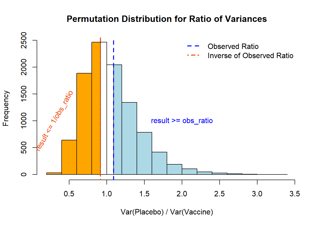
First, let's focus on the calculation of our *observed ratio*. We know that for a permutation test p-value we need to calculate the proportion that is *as or more extreme* than what we observed. Visually, this would represent:
```{r, class.source = 'fold-hide'}
# Calculate histogram, but do not draw it
my_hist <- hist(result , plot=F)

# Color vector
my_color= ifelse(my_hist$breaks > obs_ratio, 'lightblue' , ifelse (my_hist$breaks < (1/obs_ratio)-0.2, 'orange','white' ))

# Final plot
plot(my_hist, col=my_color, border=T, xlab='Var(Placebo) / Var(Vaccine)', main='Permutation Distribution for Ratio of Variances')
rect(xleft=0.8, ybottom=0, xright=1/obs_ratio, ytop=2461, col='orange')
rect(xleft=obs_ratio, ybottom=0, xright=1.2, ytop=2042, col='lightblue')
abline( v=obs_ratio, lty=2, col='blue', lwd=2)
abline( v=1/obs_ratio, lty=4, col='orangered2', lwd=2)
legend('topright', lty=c(2,4), lwd=c(2,2), col=c('blue','orangered2'), legend=c('Observed Ratio','Inverse of Observed Ratio'), bty='n')
text(x=2, y=1000, 'result >= obs_ratio', col='blue')
text(x=0.3, y=1000, 'result <= 1/obs_ratio', col='orangered2', srt=60)
```
Numerically, these values are:
```{r}
# The correct calculations
((sum(result >= obs_ratio) + 1)/(B+1))
((sum(result <= (1/obs_ratio)) + 1)/(B+1))
```
For the two-sided p-value we then double our largest value to use for our conclusion:
```{r}
2 * max(((sum(result >= obs_ratio) + 1)/(B+1)), ((sum(result <= (1/obs_ratio)) + 1)/(B+1)))
```
If we happen to forget to check the order of our problem and we flip the direction of our inequalities we arrive at:
```{r}
# The incorrect calculations
((sum(result <= obs_ratio) + 1)/(B+1))
((sum(result >= (1/obs_ratio)) + 1)/(B+1))
2 * max( ((sum(result <= obs_ratio) + 1)/(B+1)), ((sum(result >= (1/obs_ratio)) + 1)/(B+1)))
```
We see in this case we have a nonsensical p-value that is larger than 1!! This helps us realize we may need to double check our observed statistic and how it relates to our distribution.
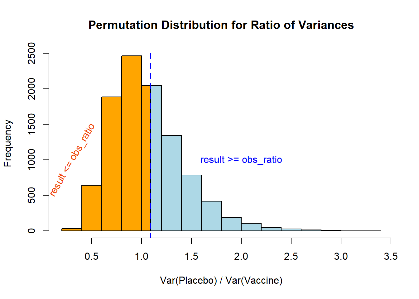
## One-Sided p-value Calculation
In the case of a one-sided p-value the approach is a little more straight forward, *but we still need to consider the context of our problem!!*
```{r, class.source = 'fold-hide'}
# Calculate histogram, but do not draw it
my_hist <- hist(result , plot=F)

# Color vector
my_color= ifelse(my_hist$breaks > obs_ratio, 'lightblue' , 'orange' )

# Final plot
plot(my_hist, col=my_color, border=T, xlab='Var(Placebo) / Var(Vaccine)', main='Permutation Distribution for Ratio of Variances')
rect(xleft=obs_ratio, ybottom=0, xright=1.2, ytop=2042, col='lightblue')
abline( v=obs_ratio, lty=2, col='blue', lwd=2)
text(x=2, y=1000, 'result >= obs_ratio', col='blue')
text(x=0.3, y=1000, 'result <= obs_ratio', col='orangered2', srt=60)
```
Here our interpretation then depends on our *a priori* specified null hypothesis (i.e., that we expect the ratio to be larger than 1 or small than 1 based on our context).
Numerically, these values are:
```{r}
# The correct calculations
((sum(result >= obs_ratio) + 1)/(B+1)) # H0 that the expected ratio > 1
((sum(result <= obs_ratio) + 1)/(B+1)) # H0 that the expected ratio < 1
```